Microsoft Sentinel 101

For people that use a lot of cloud workloads you would know it can be hard to track cost. Billing in the cloud can be volatile if you don’t keep on top of it. Bill shock is a real thing. While large cloud providers can provide granular billing information. It can still be difficult to track spend.

The unique thing about Sentinel is that it is a huge datastore of great information. That lets us write all kinds of queries against that data. We don’t need a third party cost management product, we have all the data ourselves. All we need to know is where to look.

It isn’t all about cost either. We can also also detect changes to data. Such as finding new information that can be helpful, or detect when data isn’t received.

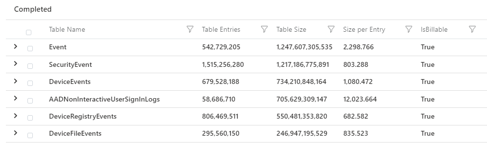
Start by listing all your tables and the size of them over the last 30 days. Query adapted from this one.

 union withsource=TableName1 *
| where TimeGenerated > ago(30d)
| summarize Entries = count(), Size = sum(_BilledSize) by TableName1, _IsBillable
| project ['Table Name'] = TableName1, ['Table Entries'] = Entries, ['Table Size'] = Size,
          ['Size per Entry'] = 1.0 * Size / Entries, ['IsBillable'] = _IsBillable
 | order by ['Table Size']  desc

You will get an output of the table size for each table you have in your workspace. We can even see if it is free data or billable.

Now table size by itself may not have enough context for you. So to take it further, we can compare time periods. Say we want to view table size last week vs this week. We do that with the following query.

let lastweek=
union withsource=_TableName *
| where TimeGenerated > ago(14d) and TimeGenerated < ago(7d)
| summarize
    Entries = count(), Size = sum(_BilledSize) by Type
| project ['Table Name'] = Type, ['Last Week Table Size'] = Size, ['Last Week Table Entries'] = Entries, ['Last Week Size per Entry'] = 1.0 * Size / Entries
| order by ['Table Name']  desc;
let thisweek=
union withsource=_TableName *
| where TimeGenerated > ago(7d)
| summarize
    Entries = count(), Size = sum(_BilledSize) by Type
| project ['Table Name'] = Type, ['This Week Table Size'] = Size, ['This Week Table Entries'] = Entries, ['This Week Size per Entry'] = 1.0 * Size / Entries
| order by ['Table Name']  desc;
lastweek
| join kind=inner thisweek on ['Table Name']
| extend PercentageChange=todouble(['This Week Table Size']) * 100 / todouble(['Last Week Table Size'])
| project ['Table Name'], ['Last Week Table Size'], ['This Week Table Size'], PercentageChange
| sort by PercentageChange desc

We run the same query twice, over our two time periods. Then join them together based on the name of the table. So we have our table, last weeks data size, then this weeks data size. Then, to make it even easier to read, we calculate the percentage change in size.

You could use this data and query to create an alert when tables increase or decrease in size. To reduce noise you can even filter on table size or percentage change. You could add the following to the query to achieve that. A small table may increase in size by 500% but is still small.

| where ['This Week Table Size'] > 1000000 and PercentageChange > 1.10

Of course, it wouldn’t be KQL if you couldn’t visualize your log source data too. You could provide a summary of your top 15 log sources with.

union withsource=_TableName *
| where TimeGenerated > ago(30d)
| summarize LogCount=count()by Type
| sort by LogCount desc
| take 15
| render piechart with (title="Top 15 Log Sources")

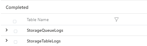
You could go to an even higher level, and look for new data sources or tables not seen before. To find things that are new in our data, we use the join operator, using a rightanti join. Rightanti joins say, show me results from the second query (the right) that weren’t in the first (the left). The following query will return new tables from the last week, not seen for the prior 90 days.

union withsource=_TableName *
| where TimeGenerated > ago(90d) and TimeGenerated < ago(7d)
| distinct Type
| project-rename ['Table Name']=Type
| join kind=rightanti 
(
union withsource=_TableName *
| where TimeGenerated > ago(7d)
| distinct Type
| project-rename ['Table Name']=Type ) 
on ['Table Name']

Let’s have a closer look at that query to break it down. Joining queries in KQL is the most challenging aspect to learn.

We run the first query (our left query), which finds all the table names from between 90 and 7 days ago. Then we choose our join type, in this case rightanti. Then we run the second query, which finds all the tables from the last 7 days. Then finally we choose what field we want to join the table on, in this case, Table Name. We tell KQL to only display items from the right (the second query), that don’t appear in the left (first query). So only show me table names that have appeared in the last 7 days, that didn’t appear in the 90 days before. When we run it, we get our results.

We can flip this around too. We can find tables that have stopped sending data in the last 7 days too. Keep the same query and change the join type to leftanti. Now we retrieve results from our first query, that no longer appear in our second.

union withsource=_TableName *
| where TimeGenerated > ago(90d) and TimeGenerated < ago(7d)
| distinct Type
| project-rename ['Table Name']=Type
| join kind=leftanti  
(
union withsource=_TableName *
| where TimeGenerated > ago(7d)
| distinct Type
| project-rename ['Table Name']=Type ) 
on ['Table Name']

Logs not showing up? It could be expected if you have offboarded a resource. Or you may need to investigate why data isn’t arriving. In fact, we can use KQL to calculate the last time a log arrived for each table in our workspace. We grab the most recent record using the max() operator. Then we calculate how many days ago that was using datetime_diff.

union withsource=_TableName *
| where TimeGenerated > ago(90d)
| summarize ['Days Since Last Log Received']  = datetime_diff("day", now(), max(TimeGenerated)) by _TableName
| sort by ['Days Since Last Log Received'] asc 

Let’s go further. KQL has inbuilt forecasting ability. You can query historical data then have it forecast forward for you. This example looks at the prior 30 days, in 12 hour blocks. It then forecasts the next 7 days for you.

union withsource=_TableName *
| make-series ["Total Logs Received"]=count() on TimeGenerated from ago(30d) to now() + 7d step 12h
| extend ["Total Logs Forecast"] = series_decompose_forecast(['Total Logs Received'], toint(7d / 12h))
| render timechart 

It doesn’t need to be all about cost either. We can use similar queries to alert on things that are new we may otherwise miss. Take for instance the SecurityAlerts table. Microsoft security products like Defender or Azure AD protection write alerts here. Microsoft are always adding new detections which are hard to keep on top of. We can use KQL to detect alerts that are new to our environment we have never seen before.

SecurityAlert
| where TimeGenerated > ago(180d) and TimeGenerated < ago(7d)
// Exclude alerts from Sentinel itself
| where ProviderName != "ASI Scheduled Alerts"
| distinct AlertName
| join kind=rightanti (
    SecurityAlert
    | where TimeGenerated > ago(7d)
    | where ProviderName != "ASI Scheduled Alerts"
    | summarize NewAlertCount=count()by AlertName, ProviderName, ProductName)
    on AlertName
| sort by NewAlertCount desc 

When we run this, any new alerts from the last week not seen prior are visible. To add some more context, we also count how many times we have had the alerts in the last week. We also bring back which product triggered the alert.

Microsoft and others add new detections so often it’s impossible to keep track of. Let KQL to the work for you. We can use similar queries across other data. Such as OfficeActivity (your Office 365 audit traffic).

OfficeActivity
| where TimeGenerated > ago(180d) and TimeGenerated < ago(7d)
| distinct Operation
| join kind=rightanti (
    OfficeActivity
    | where TimeGenerated > ago(7d)
    | summarize NewOfficeOperations=count()by Operation, OfficeWorkload)
    on Operation
| sort by NewOfficeOperations desc 

For OfficeActivity we can bring back the Office workload so we know where to start looking.

Or Azure AD audit data.

AuditLogs
| where TimeGenerated > ago(180d) and TimeGenerated < ago(7d)
| distinct OperationName
| join kind=rightanti (
    AuditLogs
    | where TimeGenerated > ago(7d)
    | summarize NewAzureADAuditOperations=count()by OperationName, Category)
    on OperationName
| sort by NewAzureADAuditOperations desc 

For Azure AD audit data we can also return the category for some context.

I hope you have picked up some tricks on how to use KQL to provide insights into your data. You can query your own data the same way you would hunt threats. By looking for changes to log volume, or new data that could be interesting.

There are also some great workbooks provided by Microsoft and the community. These visualize a lot of similar queries for you. You should definitely check them out in your tenant.