
Defenders are often looking for a single event within their logs. Evidence of malware or a user clicking on a phishing link? Whatever it may be. Sometimes though you may be looking for a series of events, or perhaps trends in your data. Maybe a quick increase in a certain type of activity. Or several actions within a specific period. Take for example RDP connections. Maybe a user connecting to a single device via RDP doesn’t bother you. What if they connect to 5 different ones in the space of 15 minutes though? That is more likely cause for concern.
If you send a lot of data to Sentinel, or even use Microsoft 365 Advanced Hunting, you will end up with a lot of information to work with. Thankfully, KQL is amazing at data summation. There is actually a whole section of the official documentation devoted to aggregation. Looking at the list it can be pretty daunting though.

The great thing about aggregation with KQL in Log Analytics is that you can re-apply the same logic over and over. Once you learn the building blocks, they apply to nearly every data set you have.
So let’s take some examples and work through what they do for us. To keep things simple, we will use the SecurityAlert table for all our examples. This is the table that Microsoft security products write alerts to. It is also a free table!
count() and dcount()
As you would expect count() and dcount() (distinct count) can count for you. Let’s start simple. Our first query looks at our SecurityAlert table over the last 24 hours. We create a new column called AlertCount with the total. Easy.
SecurityAlert
| where TimeGenerated > ago(24h)
| summarize AlertCount=count()
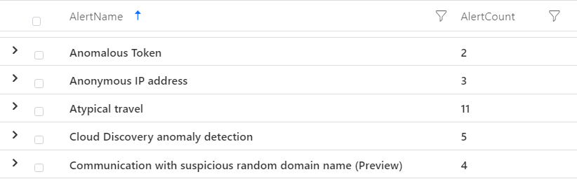
To build on that, you can count by a particular column within the table. We do that by telling KQL to count ‘by’ the AlertName.
SecurityAlert
| where TimeGenerated > ago(24h)
| summarize AlertCount=count() by AlertName
This time we are returned a count of each different alert we have had in the last 24 hours.
You can count many columns at the same time, by separating them with a comma. So we can add the ProductName into our query.
SecurityAlert
| where TimeGenerated > ago(24h)
| summarize AlertCount=count() by AlertName, ProductName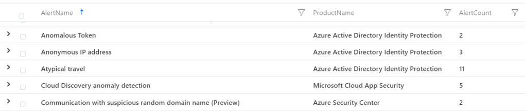
We get the same AlertCount, but also the product that generated the alert.
For counting distinct values we use dcount(). Again, start simply. Let’s count all the distinct alerts in the last 24 hours.
SecurityAlert
| where TimeGenerated > ago(24h)
| summarize DistinctAlerts=dcount(AlertName)
So in our very first query we had 203 total alerts. By using dcount, we can see we only have 41 distinct alert names. That is normal, you will be getting multiples of a lot of alerts.
We can include ProductName into a dcount query too.
SecurityAlert
| where TimeGenerated > ago(24h)
| summarize DistinctAlerts=dcount(AlertName) by ProductName
We are returned the distinct alerts by each product.
To build on both of these further, we can also count or dcount based on a time period. For example you may be interested in the same queries, but broken down by day.
SecurityAlert
| where TimeGenerated > ago(7d)
| summarize AlertCount=count() by bin(TimeGenerated, 1d)
So let’s change our very first query. First, we look back 7 days instead of 1. Then we will put our results into ‘bins’ of 1 day. To do that we add ‘by bin(TimeGenerated, 1d)’. We are saying, return 7 days of data, but put it into groups of 1 day.

If we include our AlertName, we can still do the same.
SecurityAlert
| where TimeGenerated > ago(7d)
| summarize AlertCount=count() by AlertName, bin(TimeGenerated, 1d)
We see our different alerts placed into 1 day time periods. Of course, we can do the same for dcount.
SecurityAlert
| where TimeGenerated > ago(7d)
| summarize AlertCount=dcount(AlertName) by bin(TimeGenerated, 1d)
Our query returns distinct alert names per 1 day blocks.
countif() and dcountif()
The next natural step is to look at countif() and dcountif(). The guidance for these states “Returns a count with the predicate of the group”. Well, what does that mean? It’s more simple that it seems. It means that it will return a count or dcount when something is true. Let’s use our same SecurityAlert table.
SecurityAlert
| where TimeGenerated > ago(1d)
| summarize HighSeverityAlerts=countif(AlertSeverity == "High")
In this query, we look for all Security Alerts in the last 24 hours. But we want to only count them when they are high severity. So we include a countif statement.

When we ran this query originally we had 203 results. But filtering for high severity alerts, we drop down to 17. You can include multiple arguments to your query.
SecurityAlert
| where TimeGenerated > ago(1d)
| summarize HighSeverityAlerts=countif(AlertSeverity == "High" and ProductName == "Azure Active Directory Identity Protection")
This includes only high severity alerts generated by Azure AD Identity Protection. You can countif multiple items in the same query too.
SecurityAlert
| where TimeGenerated > ago(1d)
| summarize HighSeverityAlerts=countif(AlertSeverity == "High"), MDATPAlerts=countif(ProductName == "Microsoft Defender Advanced Threat Protection")
This query returns two counts. One for high severity alerts and the second for anything generated by MS ATP. You can break these down into time periods too, like a standard count. Using the same logic as earlier.
SecurityAlert
| where TimeGenerated > ago(7d)
| summarize HighSeverityAlerts=countif(AlertSeverity == "High") by bin(TimeGenerated, 1d)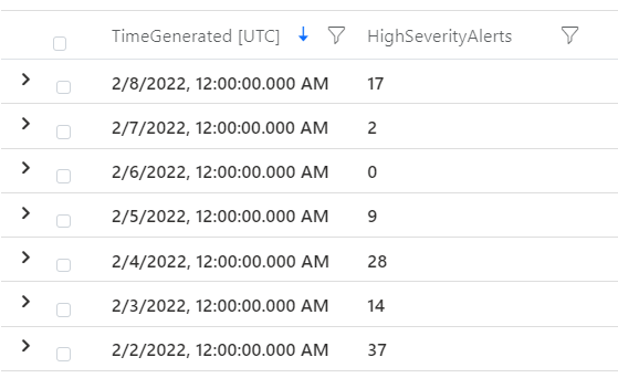
We see high severity alerts per day over the last week.
dcountif works exactly as you would expect too. It returns a distinct count where the statement is true.
SecurityAlert
| where TimeGenerated > ago(24h)
| summarize DistinctAlerts=dcountif(AlertName, AlertSeverity == "High")
This will return distinct count of alert names where the alert severity is high. And once again, by time bucket.
SecurityAlert
| where TimeGenerated > ago(7d)
| summarize DistinctAlerts=dcountif(AlertName, AlertSeverity == "High") by bin(TimeGenerated, 1d)
arg_max() and arg_min()
arg_max and arg_min are a couple of very simple but powerful functions. They return the extremes of your query. Let’s use our same example query to show you what I mean.
SecurityAlert
| where TimeGenerated > ago(1d)
| summarize arg_max(TimeGenerated, *)
If you run this query, you will be returned a single row. It will be the latest alert to trigger. If you had 500 alerts in the last day, it will still only return the latest.
arg_max tells us to retrieve the maximum value. In the brackets we select TimeGenerated as the field we want to maximize. Then our * indicates return all the data for that row. If we switch it to arg_min, we would get the oldest record.
We can use arg_max and arg_min against particular columns.
SecurityAlert
| where TimeGenerated > ago(1d)
| summarize arg_max(TimeGenerated, *) by AlertName
This time we will be returned a row for each alert name. We tell KQL to bring back the latest record by Alert. So if you had the same alert trigger 5 times, you would just get the latest record.
These are a couple of really useful functions. You can use it to calculate when certain things last happened. If you look up sign in data and use arg_max, you can see when a user last signed in. Of if you were querying device network information. Querying the latest record would return you the most up to date information.
You can use your time buckets with these functions too.
SecurityAlert
| where TimeGenerated > ago(30d)
| summarize arg_max(TimeGenerated, *) by AlertName, bin(TimeGenerated, 7d)
With this query we look back 30 days. Then for each 7 day period, we return the latest record of each alert name.

make_list() and make_set()
make_list does basically what you would think it does, it makes a list of data you choose. We can make a list of all our alert names.
SecurityAlert
| where TimeGenerated > ago(1d)
| summarize AlertList=make_list(AlertName)
What is the difference between make list and make set? Make set will only return distinct values of your query. So in the above screenshot you see ‘Unfamiliar sign-in properties’ twice. If you run –
SecurityAlert
| where TimeGenerated > ago(1d)
| summarize AlertList=make_set(AlertName)
Then each alert name would only appear once.
Much like our other aggregation functions, we can build lists and sets by another field.
SecurityAlert
| where TimeGenerated > ago(1d)
| summarize AlertList=make_list(AlertName) by AlertSeverity
This time we have a list of alert names by their severity.
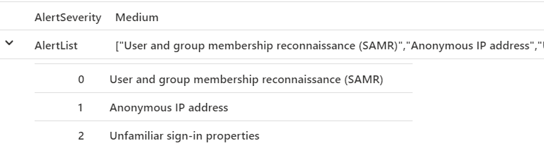
Using make_set in the same query would return distinct alert names per severity. It won’t shock you if you are still reading to know that we can make lists and sets per time period too.
SecurityAlert
| where TimeGenerated > ago(7d)
| summarize AlertList=make_set(AlertName) by bin(TimeGenerated, 1d)
This query gives us a list of alert names per day over the last 7 days. And the same to make a set.
SecurityAlert
| where TimeGenerated > ago(7d)
| summarize AlertList=make_set(AlertName) by AlertSeverity, bin(TimeGenerated, 1d)
make_list_if() and make_set_if()
make_list_if() and make_list_if() are the natural next step to this. They create lists or sets based on a statement being true.
SecurityAlert
| where TimeGenerated > ago(1d)
| summarize AlertList=make_list_if(AlertName,AlertSeverity == "High")
For example, build a list of alert names when the severity is high.

When we do the same but with make_set, we see we only get distinct alert names.
SecurityAlert
| where TimeGenerated > ago(1d)
| summarize AlertList=make_list_if(AlertName,AlertSeverity == "High")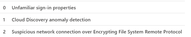
This supports multiple parameters and using time blocks too of course.
SecurityAlert
| where TimeGenerated > ago(7d)
| summarize AlertList=make_set_if(AlertName,AlertSeverity == "Medium" and ProductName == "Microsoft Defender Advanced Threat Protection") by bin(TimeGenerated, 1d)
This query creates a set of alert names for us per day. But it only returns results where the severity is medium and the alert is from MS ATP.
Visualizing your aggregations
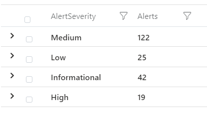
Now the really great next step. Once you have summarized your data you can very easily build really great visualizations with it. First, lets summarize our alerts by their severity
SecurityAlert
| where TimeGenerated > ago(1d)
| summarize Alerts=count()by AlertSeverity
Easy, that returns us a summarized set of data.
Now to visualize that in a piechart, we just add one simple line.
SecurityAlert
| where TimeGenerated > ago(1d)
| summarize Alerts=count()by AlertSeverity
| render piechart 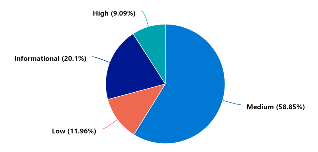
KQL will calculate it and build it our for you.
For queries you look at over time, maybe a timechart or columnchart makes more sense.
SecurityAlert
| where TimeGenerated > ago(7d)
| summarize Alerts=count()by AlertSeverity, bin(TimeGenerated, 1d)
| render timechart 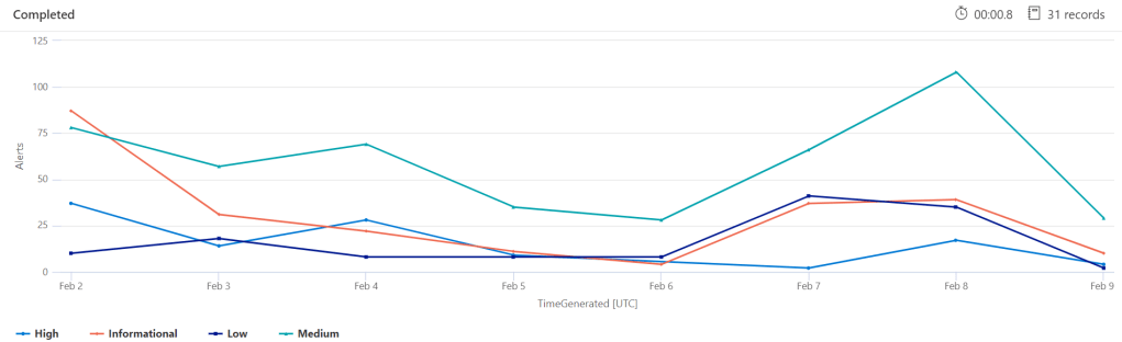
You can see the trend in your data over the time you have summarized it.
Or as a column chart.
SecurityAlert
| where TimeGenerated > ago(7d)
| summarize Alerts=count()by AlertSeverity, bin(TimeGenerated, 1d)
| render columnchart 
KQL will try and guess axis titles and things for you, but you can adjust them yourself. This time we unstack our columns, and rename the axis and title.
SecurityAlert
| where TimeGenerated > ago(7d)
| summarize Alerts=count()by AlertSeverity, bin(TimeGenerated, 1d)
| render columnchart  with (kind=unstacked, xtitle="Day", ytitle="Alert Count", title="Alert severity per day")
Aggregation Examples
Interested in aggregating different types of data? A couple are listed below.
This example looks for potential RDP reconnaissance activity.
DeviceNetworkEvents
| where TimeGenerated > ago(7d)
| where ActionType == "ConnectionSuccess"
| where RemotePort == "3389"
// Exclude Defender for Identity which uses RDP to map your network
| where InitiatingProcessFileName <> "Microsoft.Tri.Sensor.exe"
| summarize RDPConnections=make_set(RemoteIP) by bin(TimeGenerated, 20m), DeviceName
| where array_length(RDPConnections) >= 10
We can break this query down by applying what we have learned. First we write our query to look for the data we are interested in. In this case, we look at 7 days of data for successful connections on port 3389. Then we use one of our summarize functions. We make a set of the remote IP addresses each device is connecting to, and place that data into 20 minute bins. We know that each remote IP addresses will be distinct, because we made a set, not a list. Then we look for devices that have connected to 10 or more IP’s in a 20 minute period.
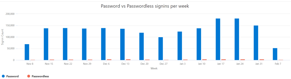
Have you started your passwordless journey? You can visualize your journey using data aggregation.
SigninLogs
| project TimeGenerated, AuthenticationDetails
| where TimeGenerated > ago (90d)
| extend AuthMethod = tostring(parse_json(AuthenticationDetails)[0].authenticationMethod)
| where AuthMethod != "Previously satisfied"
| summarize
    Password=countif(AuthMethod == "Password"),
    Passwordless=countif(AuthMethod in ("FIDO2 security key", "Passwordless phone sign-in", "Windows Hello for Business"))
    by bin(TimeGenerated, 7d)
| render columnchart
    with (
    kind=unstacked,
    xtitle="Week",
    ytitle="Signin Count",
    title="Password vs Passwordless signins per week")
We look back at the last 90 days of Azure AD sign in data. Then use our countif() operator to split out password vs passwordless logins. Then we put that into 7 day buckets, so you can see the trend. Finally, build a nice visualization to present to your boss to ask for money to deploy passwordless. Easy.
A few other useful sites around data aggregation.

One thought on “Too much noise in your data? Summarize it!”
1 Pingback